
Model Sensitivity Analysis
When it comes to finance, a model can be as reliable as its premises. There is uncertainty in revenue forecasts, in the discount rates, and in the operating cost ratios – all of these contain uncertainty, and when you put a combination of several uncertain assumptions together, chances are that the final output will swing wildly depending on the conditions that are beyond your control. That is precisely why sensitivity analysis in financial modeling has dawned on as one of the most crucial skills of finance professionals at each and every organisational level.
Sensitivity analysis refers to the process of testing how varying the input variables of a model can change the model’s output – usually a key measure such as net present value (NPV), internal rate of return (IRR), or net profit margin. Sensitivity analysis shows the range of plausible outcomes, those assumptions most likely to be most risky, and provides insight into where decision-makers and managers should focus their attention and management effort.
This article is oriented at junior to mid-level financial professionals, business analysts and those looking at financial modeling courses in Singapore or elsewhere to whip up their quantitative skills. Whether you are making your first discounted cash flow (DCF) model or you are preparing to work in an investment banking, corporate finance, or financial planning and analysis (FP&A) role, the methods and models outlined here will provide you with a practical base in which to conduct rigorous, credible, and decision-relevant analysis.
Why Sensitivity Analysis Is Central to Sound Financial Modelling
All financial models are constructed with the help of a set of assumptions. Judgements made by analysts include future growth in revenue, as well as cost, capital expenditure, working capital and macroeconomic conditions. Each of the assumptions may appear to be reasonable in isolation. The combination of these elements, together, generates an output – an NPV, a revenue figure, a return on equity – which management and investors use to make consequential decisions. The fact is that without testing these assumptions, there is no means of knowing how weak or strong that output is.
Take an example of a manufacturing company that is considering expanding its plants by USD 200 million. Using the financial model, a positive NPV of USD 45 million at an 8% discount rate and the assumption of a 10 percent growth in revenues might be expected. However, what would happen if the global interest rate changes to 11%? Or should growth be limited to 4% by supply chain disruptions? In the absence of sensitivity analysis, the management is only presented with the rosy base case. Using it, they can learn that the project becomes NPV-negative in two plausible situations – and they can make plans based on that.
In addition to risk identification, sensitivity analysis enhances the level of financial communication. Whenever a CFO is making a business case to the board, stakeholders will always ask him/her what if questions. Being able to answer such questions confidently and transparently, as opposed to stumbling around trying to find answers in the middle of the meeting. That is why sensitivity analysis in financial modeling is continuously considered as one of the core competencies in the finance job description worldwide.
The Five Key Steps to Conducting a Robust Sensitivity Analysis
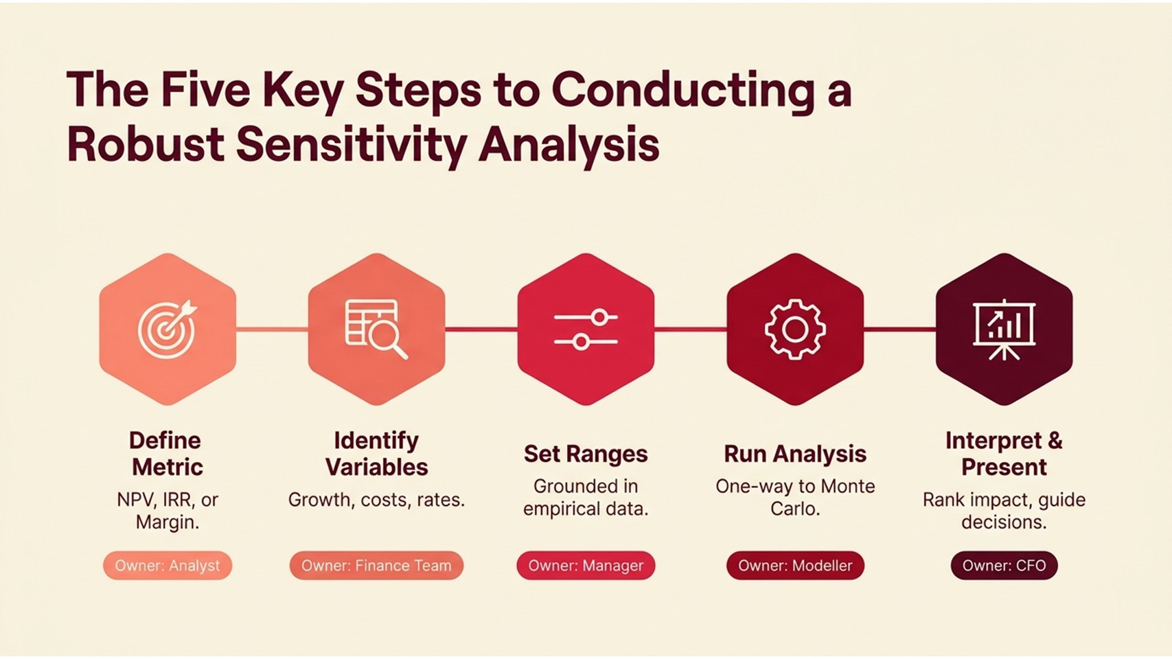
Though the software tools and complexity of models vary, the underlying methodology of sound sensitivity analysis conforms to a basic five-step process. The following process flow may be used by analysts in any industry, whether it is real estate development or a project evaluation of a technology project.
| Phase | Action | Owner |
| Step 1 | Specify the Metric of the Output.
Determine which KPI to measure – NPV, IRR, gross margin or free cash flow. |
Financial Analyst |
| Step 2 | Determine important input variables.
Enumerate all assumptions that lead to the output: growth rates, costs, discount rates, and volumes. |
Finance Team |
| Step 3 | Set Variable Ranges
Give each input realistic low, base, and high values based on a past or benchmark. |
Senior Analyst / Manager |
| Step 4 | Run the Analysis
Modify one or many inputs ( one-way or Monte Carlo ). |
Financial Modeller |
| Step 5 | Interpret Results & Communicate
Prioritize variables of impact, create charts (tornado/spider), and share the results with stakeholders. |
Finance Manager / CFO |
The initial one – the definition of the output measure – is a more subtle thing than it may seem. There can be many KPIs related to a single model: NPV to make capital allocation decisions, IRR to compare with a hurdle rate, and payback period to be liquidity-conscious. It is best to select the appropriate metric of output early in the analysis to ensure that the analysis is focused and actionable as opposed to producing a diffuse set of results about which no one knows what to do.
Analyst judgment is most vital in identifying a range of input variables. The best practice is to utilize historical data, assuming that the historical data is available, for at minimum three or five years to understand the variability of each assumption in real-life. To a retail business, revenue growth could have been between -3% and +18% in a 10-year time period. In the case of a utility company, it could be much more limited. One of the most significant sensitivity analysis best practices that you can embrace is basing your ranges on empirical evidence, as opposed to relying on gut feeling.
Types of Sensitivity Analysis: From Simple to Sophisticated

There is no equality when it comes to creating sensitivity analysis. The decision complexity, data accessibility, and the audience to whom the results will be presented are some of the factors that should be considered when deciding which type to use. The most typical place to start is a one-way sensitivity analysis. It entails varying one input variable over a range of values whilst keeping all the other inputs at constant values. The results – a tornado chart (typically) of the output, with the variables listed by rank of the size of their NPV impact.
Table 1: Scenario Output Comparison — Infrastructure Project Evaluation
| Scenario | Revenue Growth | EBITDA Margin | Project NPV (USD M) |
| Base Case | 8% | 22% | 120 |
| Optimistic | 14% | 27% | 185 |
| Pessimistic | 2% | 15% | 62 |
| Stress Test | -5% | 9% | –31 |
Two-way sensitivity analysis generalizes this by considering two inputs combined and giving results in a data table matrix – for example, showing NPV at each combination of revenue growth (rows) and discount rate (columns). This is especially beneficial when it comes to exploring the effects of interaction. A project may be feasible with a high growth rate and a high discount rate, but not with a moderate growth rate and a small increase in the discount rate. These threshold relationships are clearly brought out in two-way tables.
Table 2: Input Variable Sensitivity Ranking — Consumer Goods Expansion Model
| Input Variable | Range Tested | NPV Impact (USD M) | Sensitivity Rank |
| Revenue Growth Rate | –5% to +14% | ±63 | 1st |
| Discount Rate (WACC) | 7% to 13% | ±41 | 2nd |
| Operating Cost Ratio | 55% to 75% | ±28 | 3rd |
| Tax Rate | 17% to 25% | ±14 | 4th |
| Capex Intensity | ±10% of base | ±9 | 5th |
The state of the art of sensitivity analysis is Monte Carlo simulation. Instead of using discrete high/low values, Monte Carlo methods make use of probability distributions to each input and perform thousands of simulated iterations, resulting in a distribution of output outcomes. This is particularly useful in large capital projects, infrastructure investment or developing a pharmaceutical programme where the uncertainty of cost and timeline is many-dimensional and variables interdepend heavily. Monte Carlo modules are frequently found as part of higher-level quantitative finance programs, and are often studied as part of financial modeling courses in Singapore.
Real-World Applications and Lessons Learned
In order to demonstrate how sensitivity analysis works in reality, we will take an example of a mid-sized European retail chain considering an entry into three new markets at the same time. The first model had an interesting consolidated IRR of 19% – higher than the 15% hurdle rate of the group. Nevertheless, when the finance team performed a one-way sensitivity analysis, they found that the IRR was below the hurdle rate, in case same-store sales growth decreased to below 6%, which was only surpassed in two of the last eight years in similar markets.
The sensitivity analysis failed to slay the project. Rather, it reformulated the decision. The management decided to only venture into one market first and treat it as a pilot that would either prove (or dispel) the expansion premises before capitalizing on the other two markets. This gradual strategy, proactively informed by the sensitivity output, saved about USD 80 million in capital that would have been deployed under dubious assumptions. The lesson: sensitivity analysis is not simply a reporting tool; it is a strategic decision-making tool.
A second example is a modelling exercise by an energy company to model the economics of a renewable power project. The first model assumed the power purchase agreement (PPA) tariff to be fixed and sensitivity testing was almost solely on the cost of construction and capacity factors. In a peer review, a senior analyst said that there was the risk of regulatory renegotiation of the PPA tariff itself, a variable that had not been modeled at all in the sensitivity framework. A 12 percent tariff cut when it was introduced and tested rendered the project NPV negative. The case exemplifies yet another of the most frequently mentioned sensitivity analysis best practices: never assume that you have listed all variables you may be interested in. Question the assumptions on which the assumptions are based.
Common Challenges and How to Overcome Them
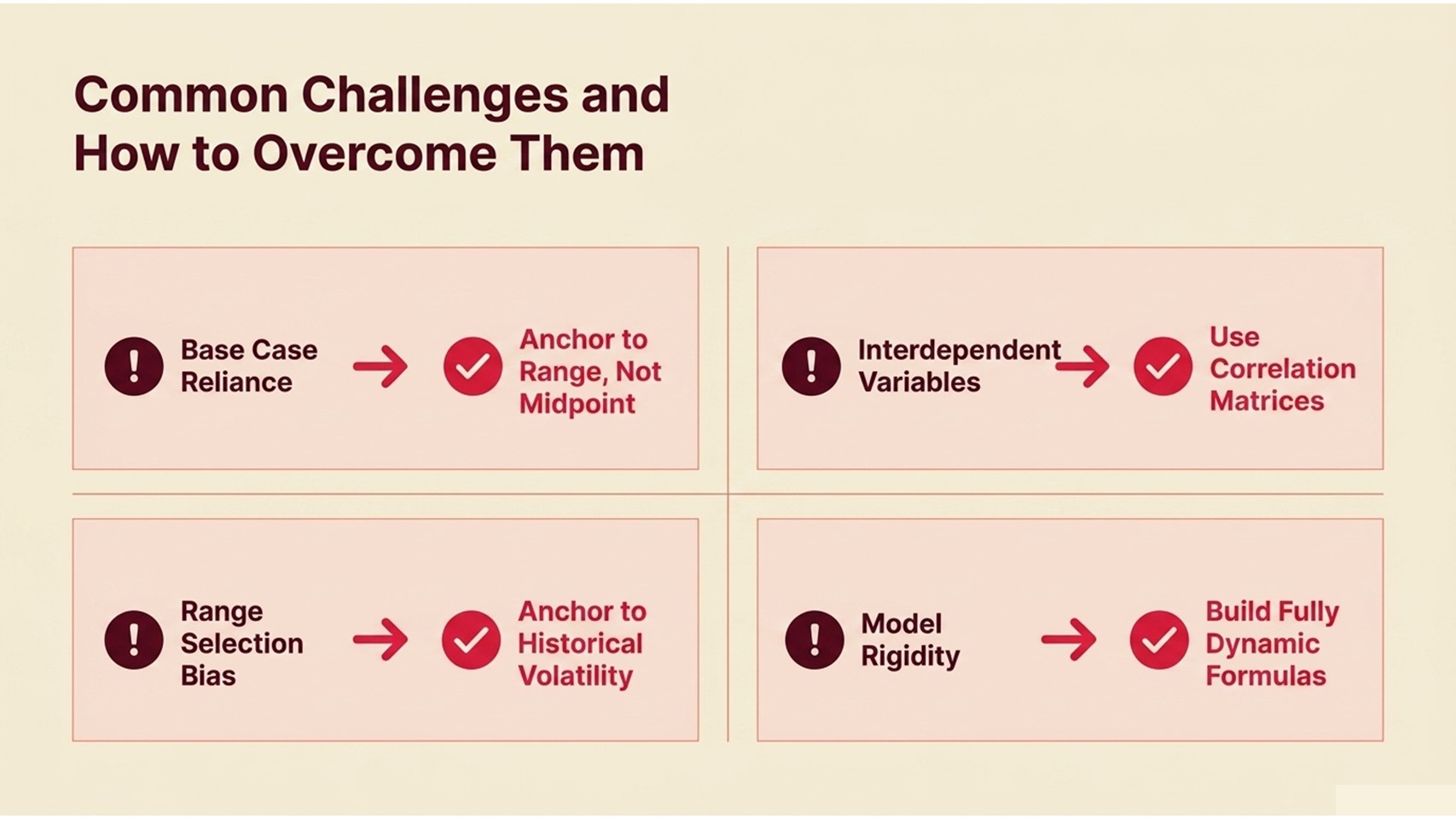
Even though it is a valuable technique, sensitivity analysis is often poorly applied in practice. The following are some of the challenges that are real, recurring and avoidable, provided you know what to look at. The following process table will map each challenge to its root cause and a suggested mitigation strategy.
Process Flow 2: Common Sensitivity Analysis Challenges and Mitigations
| Common Challenge | Why It Occurs | Recommended Mitigation |
| Oversensitivity to Base Case. | The base case is taken as certainty and the results of scenarios are disregarded by the stakeholders. | Always have three scenarios, and anchor the communication based on the range and not the midpoint. |
| Interdependent Variables | When one of the many inputs (e.g., price) is changed, one or more of the other inputs (e.g., volume) is inevitably affected, distorting one-way tests. | Simulate dependencies among variables with the use of correlation matrices or Monte Carlo simulations. |
| Range Selection Bias | Analysis: Narrow ranges are selected by analysts to reduce the apparent risk, and thus the model is misleading. | Anchor ranges to historical volatility or third-party standards; get a peer review of the ranges. |
| Model Rigidity | Formulas Hard-coded formulas are used when the ranges change, causing errors or incorrect results. | Construct completely dynamic models with the input cells clearly labelled; first, stress-test the model structure. |
| Poor Visualisation | Raw sensitivity tables are not easy to read; decision-makers do not get important insights. | Tornado charts should be used to perform one-way analysis, and scenario dashboards to present multi-variable presentations. |
Among the challenges that should be mentioned in particular, there is the temptation to reverse-engineer the sensitivity ranges to support a predetermined conclusion. This is not an exception, as most professionals would want to admit. When a project sponsor is aware that the NPV is negative at an increase in the discount rate up to a 5 percent level, then he could put the high discount rate in the sensitivity table to a value of just a bit below the break-even point at 4.5 percent. The best practices of rigorous sensitivity analysis require ranges to be established prior to running the analysis and that the analysis methodology should be documented and should be reviewable by a third party.
Communication is another challenge that is often undermined. An ideal sensitivity analysis in the form of a thick spreadsheet will never make a difference to a boardroom decision. Investments made in clear visualisation (tornado charts, scenario dashboards, written executive summaries) are always reported to have increased the uptake of their analytical work by finance professionals. The insight can only be valuable when it gets to and is comprehended by the decision-maker.
Conclusion: Building Sensitivity Analysis Into Your Finance Toolkit
Sensitivity analysis is not an incidental, optional add-on to financial modelling – it is a fundamental part of a decision-relevant financial analysis. The methodology, which moves up the ladder of importance of variables by one-way tests to the full Monte Carlo simulations of probability outcomes, is scaled to the complexity of any decision environment. What is constant in all applications is the inherent purpose, that is, to substitute false certainty with honest uncertainty, and to provide decision-makers with the information they need to act wisely under conditions they are not able to fully control.
To those just starting their finance careers, the most valuable thing is to inculcate the habit of sensitivity analysis in every model that you create – even simple ones. Begin with a test, one-way, on two or three of the most significant assumptions. Communicating the results of a tornado chart is best done using a tornado chart. Record your range-setting procedure. These will turn into habits, and in the long run, your models will become significantly more believable to the stakeholders.
To individuals interested in developing their technical skills, formal programmes such as the financial modeling courses Singapore offer practical training in developing dynamic sensitivity frameworks, scenario analysis and the application of Monte Carlo simulation using industry standard tools. Formal training coupled with practice is the quickest way to become proficient.
The most distinguished representatives of the profession of finance are not those who create the most elaborate models – they are those whose models most consistently help to make better decisions. Learning to perform sensitivity analysis financial modeling, and do so with the best practices, is by and large one of the simplest approaches to becoming that professional. Begin with the following model you make. Test the assumptions. Challenge the ranges. Communicate the uncertainty. And make the analysis what it is meant to be: rigorous and sane in making decisions that count.